Realtime Covid-19 spread modelling

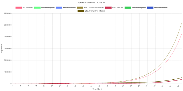
This is an upgrade to the previous project. Instead of taking hypothetical values for the SIR model parameters, this program retrieves the latest (daily) time series data for the Coronavirus pandemic from https://pomber.github.io/covid19/timeseries.json and simulates how the infection might play out in the future. The time series data is used to get an estimate of the SIR parameters β (the "contact rate" constant) and α (recovery constant). These vary enough through time to cause wild variations in the model outcome. So, I've included the option to use the latest, the minimum, the maximum and the mean values, out of which the mean seems to give the most sensible looking graph. The way the parameters are estimated is basically using two (shorter) of the three governing equations of the model:
delS/delT = -β*S*I/N
delI/delT = β*S*I/N - α*I
delR/delT = α*I
from where,
β = delS/(I*S/N)
α = delR/I
where delT = 1 day, since that is how frequent the available data is.
Now, the Susceptible population S, Infective population I and the Removed population R aren't available as such. The time series data source mentioned above gives the daily recorded data for each country since Feb. 22, 2020. This is converted into a global daily record time series data by summing over all the countries. The final form looks something like this, and this is for a particular date:

1. date: "2020-3-26"

1. confirmed: 529591

1. deaths: 23970

1. recovered: 122149

The 'confirmed' value corresponds to all the active infections (which meets the definition of the infective population in our model) + the 'deaths' + the 'recovered' values.

So, for the infective population, I = confirmed -  deaths - recovered

and for the susceptible population, that's the global population minus the people who are still in active infection and those who've recovered or died combined i.e. S = N - confirmed

I tried doing a simple power-law function fitting for the alpha and beta parameters using the Least Square Technique (LST) here but ultimately decided against using it in the model as I thought their time-evolution should be more logistic-like rather than monotonous. For that spreadsheet, I used data attributed to Mathemaniac after watching his video

Perhaps I could use the latest 5-day or 14-day averages for better estimating the model parameters. The model would do even better if I could figure out β(t) and α(t) for the entire duration of the epidemic since the parameters seem to be constantly fluctuating IRL.

Anyway, here is the code.

Edit: I've removed the (flawed) max/min parameter estimation and added last 5 and last 14 data based parameter estimation. Doesn't seem to do much good.
Edit: I've only now realized that web apps that don't require/have a back end i.e. web pages that don't require server-side coding can be hosted on GitHub itself! I have thus pushed this project to GitHub as a repository. The corresponding GitHub Pages site is here. I will be pushing all future JavaScript web apps directly to GitHub as repositories of their own; no more GitHub Gist for such programs. All update to the apps will be applied to their corresponding GitHub repositories, not their Gists. I will also be shortly porting all my past JavaScript web apps in this blog that I'd uploaded to GitHub Gist to GitHub as repositories.

Epidemic Spread Modelling with the SIR model

The recent national lockdown due to the Covid-19 global pandemic has afforded me all the free time in the world. So, I took this opportunity to learn more about how experts study epidemics to make inferences and devise policies. I inquired Google and YouTube on the topic and quickly discovered a wealth of relevant resources. Books, papers, articles and videos were aplenty. Herbert W. Hethcote (Three Basic Epidemiological Models), Aresh Dadlani et. al. (Deterministic Models in Epidemiology: from Modeling to Implementation), Fred Brauer and Carlos Castillo-Chávez (Epidemic Models) and Yiran Jing were the authors whose work I found really helpful in understanding how epidemic modelling works. YouTube videos from channels: Trefor Bazett, Tom Rocks Maths and VetenskapensHus were veritable gems on the subject owing to their platform-incentivized conciseness. Anyway, back to SIR - this model is arguably the simplest of all while still being able to yield useful insights into the workings of an epidemic.
There are two variants of the model - with and without vital dynamics (birth, death, migration). Here, I deal with the no vital dynamics variant which basically implies there's no significant change in the total population of the community under study, at least until the epidemic lasts. The idea is, the population is divided into three categories - Susceptible (normal, not yet infected individuals), Infective (infected individuals, who can infect others) and Recovered/Removed (individuals who have recovered from the disease and will not again go back to being infected, say because they've gained immunity). Populations of each compartment are constantly changing, moving from Susceptible(S) to Infective(I) to Recovered(R). The flux or rate of change of the population of each compartment (dS/dt, dI/dt, dR/dt) is assumed to be functions of one or multiple of such categorical populations. For example, the rate at which S changes into I is assumed to be proportional to the product of the Infective population and the Susceptible population. Such an ODE is written down for each of the compartments - giving a total of 3 ODEs that have to be solved simultaneously while satisfying the constant population assumption(S+I+R=N=constant). The system of ODEs happens to be impossible to solve explicitly owing to non-linearities in two of the three equations. So, only numeric solutions for I, S and R as functions of time are possible, via discretization as per the ole'faithful Finite Difference Method, which is what I've done here. The details of the model can be found on any of the resources listed above.
Here's how the graphs look:

Here's the code.
EDIT:
This is after I've realized what GitHub Pages is.
Live demo here
Corresponding repo here
Future updates, if any, will be made to the repo, not the Gist

Riverbed variation model

I haven't been able to manage enough time to code lately. It has got to do with me starting a job - out of a necessity of - I don't know what. But more on that on my other blog (that I hope I do write). Anyway, I thought I should put it here for my own sense of continuity rather than for the (dys)functionality slash (un)greatness of this code.

This is a problem that has to do with predicting the evolution of riverbed elevations in sediment carrying rivers. Yeah, also part of the (second semester of) M.Sc. Water Resources Engineering program's Water Induced Hazards::Riverbed Variation(RBV) module.
The problem of scraping together enough time to invest in writing a functioning program aside, this physical process inherently seems to me so very intractable to put into a working model, even now, when I believe I have a somewhat acceptable result it spit out a few minutes ago which was when I decided to do this write-up. What the program does is solve three PDEs describing the phenomenon using the much acclaimed MacCormack explicit finite differencing scheme.
When the equations were first presented in class, I don't believe there was much explanation regarding what each term meant  in a physical sense, and more importantly, how one interacted with  others. The presentation went something like this: write down the PDEs; discretize them to obtain equations for the next time level's riverbed elevation, water depth and specific discharge; write down the CFL condition; try and work out a numerical problem. So many questions were left unanswered: What should the boundary conditions be? Are they important? How sensitive is the output to boundary conditions? What does the sediment transport equation relating specific sediment discharge(qs) with specific discharge(q) mean? What does it mean to solve for specific discharge? Does specific discharge itself change as a result of riverbed variation? What output am I expecting? How should the computation procedure move in the finite difference grid? And as I put pen to paper, so to speak, there were so many possibilities to try - each requiring a great deal of effort - while most likely being wrong. One would easily be forgiven for giving up on even trying. Anyway, cut long story short, I tried to get it to work - a lot - and failed - a lot. Until I stumbled upon this article that referenced

Alam M (1998) Application of MacCormack scheme to the study of aggradation degradation in alluvial channels M.Sc. Engineering thesis work, Department of Water Resources Engineering, BUET, Dhaka.

 available here. The "Full thesis" was freely available for download at the second link. The document proved extremely helpful and answered most of my questions. It also detailed a set of controlled lab experiments on RBV and gave me a sense of what I should be expecting from my program.
So, here is what the program does:
1. Takes in all the relevant input parameters.
2. Populates the first element of an array of "profile"objects. The first object in this array has the initial condition values for h, q and z along with x and t. x is an array of downstream nodal points. h, q and z are arrays of water depths, specific discharges and bed elevations at their respective x positions. t is the time level of the profile.
3. Runs a loop from 0 to the stipulated maximum time of simulation. For each iteration of this loop, there's another loop for computing the next time level's h, q and z values using the MacCormack explicit formulae at all downstream nodes.
4. The sediment discharge at the first (zero) node is held at a constant value that is a user-specified multiple of the sediment carrying capacity(?) of the initial flow [i.e. qs=a(q/h)^b] for all time levels. So is the water discharge.
5. Displays the final profiles in a graph as an animation.
While in algorithm, the process seems pretty straightforward, there are subtleties involved to say the least in the actual implementation in code. The MacCormack scheme needs values of the unknown parameters one spatial node in excess to the up and downstream while time-marching from any node. This necessitates calculations of parameters in as many nodes downstream of the actual downstream boundary as the number of time levels desired. For nodes requiring info from upstream of the upstream boundary, the respective initial state values are assigned i.e. no fictitious nodes black magic is performed.
Also, keeping track of the profiles at different time levels and using the right ones in the scheme without screwing up in the slightest is easier said than done.
There is also the coordination between the main and the WebWorker thread and figuring out a good dynamic between the two.
Not all input parameters output a good result. In fact, most inputs lead to an explosion of the predicted parameters at some point in time. I've tried decreasing delT thinking it may be a manifestation of the scheme's instability because the CFL condition may have been violated. But even when there's a more than comfortable buffer between the used delT and the threshold between that predicted by the Courant condition, I've seen irrational predictions owing to negative q's, tiny q's and what not. While the aforementioned paper recommends using a new delT after each time march depending on the new q and h values using the CFL criterion, I'm skeptical it would offer any significant improvements.
Anyway, I'm done with this.
EDIT:
This is after I've realized what GitHub Pages is.
Live demo here
Corresponding repo here
Future updates, if any, will be made to the repo, not the Gist

I don't know why the first time march reduces the bed level to below the initial value here.